Understanding the Distribution
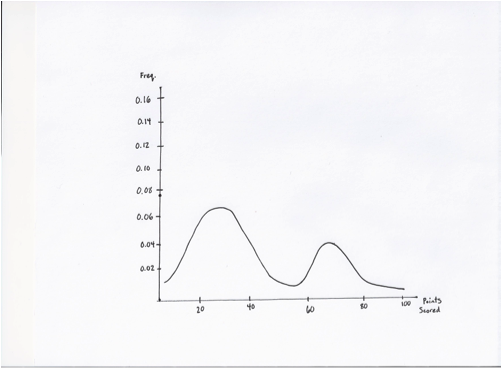
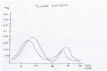
As you can see, the Scrabble distribution is largely Gaussian, but with two humps: one bell curve representing the score of the non-bingo plays, while the other bell curve represents the score of bingos. Entropy is represented by the point differences between both curves, and can often be approximated by the difference between the local maxima.
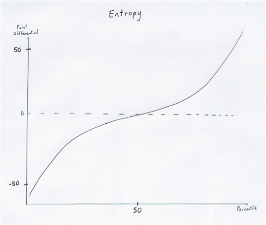
This graph represents the difference in entropy given a standard Scrabble distribution. As you can see, the point difference between you and your opponent on an average board is quite high. Approximately 1/3 of the time, when we use this method, one player will bingo and the other will not, resulting in a fairly large point swing.
This graph represents the effect of entropy over one turn. As you can see, there is a high potential of a significant points swing, either by your or by your opponent: whether you are ahead or behind by 40 points, you can easily be behind on your next turn.
Examples:
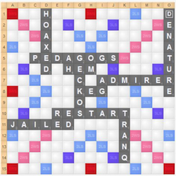 |  |
This is an example of an open board with a low entropy. Here, there are many scoring and bingo opportunities, and the bingo opportunities are not far outweighed by the scoring opportunities: thus, it can be difficult to make up a large lead.
This is an example of an entropic open board. Here, there are plenty of bingo lines available but the opportunities are much more for bingos than scoring, as it is difficult to score with high point tiles on this board.
This is an example of a typical closed board. There are a few scoring options available but not much in terms of bingo options, and swings in this game will be fairly minimal.